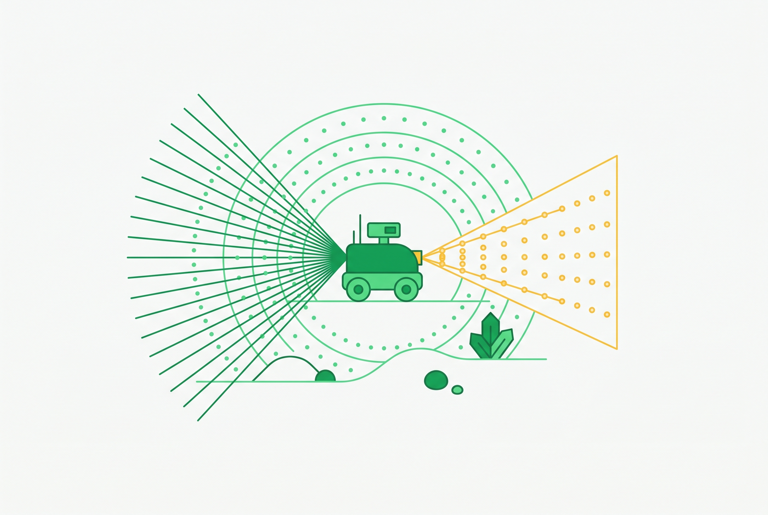
ROS 2 Nav2 Stack Configuration for Outdoor Uneven Terrain

Outdoor uneven-terrain configuration for ROS 2 Nav2 is an exercise in compensating for a 2D planning abstraction. Reliable operation depends on matching costmap layers, terrain classification, localization, and planning to that constraint. Those choices can work for many outdoor routes, but they cannot provide genuine 3D planning and need regular field maintenance to keep working.

Why Nav2's 2D planning abstraction is the root constraint, not a peripheral limitation

Nav2’s Costmap 2D represents the environment for the planner as cells with cost values from 0, meaning free, to 254, meaning lethally occupied. Although intermediate costs can express preferences, the grid cannot represent separate routes above and below a bridge or a slope that is feasible in only one direction. These are differences in path topology and directional feasibility. Projecting them into a flat grid removes information that planning would need.

Nav2 maintainers describe the stack as “widely used for navigation on planar ground” and identify 3D terrain support as a development target still under evaluation. Their criteria include production quality, broad applicability, and no massive GPU requirement. That combination sets a demanding engineering target. Until such an architecture is available, outdoor configuration must use layers and perception to turn terrain into costs the existing planner can use.

How the 2D abstraction produces specific, predictable failure modes outdoors

A navigable slope and a blocking wall can both become elevated cost cells once their geometry is flattened. Vegetation creates a related classification failure. The UC Merced ICRA 2024 work on real-time costmap updates for agricultural applications documents LiDAR treating tall grass and weeds as obstacles on a Clearpath Husky in an almond orchard. The robot consequently took longer paths or aborted navigation. The sensor detected something real, but occupancy alone did not establish whether the robot could traverse it.

Localization errors make it harder still to use that terrain information. Uneven tyre wear and changes in the surface cause systematic wheel-odometry error that an EKF cannot simply remove. Vibration on rough ground can shift sensor brackets, so the transforms in the ROS 2 TF tree no longer match where the sensors are fitted. Temperature cycling between hot pavement and cold air also changes IMU bias, progressively corrupting heading estimates. Fusion then operates on degraded measurements or incorrect geometry, even if the costmap’s obstacle classification is otherwise sound.

The outdoor environment also changes beyond a single traverse. A summer map cannot reliably describe autumn leaf piles or snow-altered traversable boundaries, so stale terrain assumptions can cause rerouting or stalls. In bright outdoor conditions, the SLAM-generated map reaches only as far as the LiDAR range allows, and goals cannot be set beyond it. Pure SLAM therefore introduces a long-distance navigation constraint that obstacle-layer tuning cannot resolve.

Choosing the right costmap layer for the sensor and compute profile available

Nav2’s official tuning guidance distinguishes costmap layers by the measurements and compute available. The practical decision starts with the sensor. ObstacleLayer suits planar LiDARs or low-compute devices because it projects 2D scan data into the costmap. It is appropriate when 3D sensing is unavailable or computational resources are severely constrained and does not retain terrain geometry. VoxelLayer accepts non-planar 2D LiDAR or depth-camera measurements and builds 3D cell occupancy, but sparse 3D LiDAR point clouds do not fill its voxels reliably.

For 3D LiDAR, the recommended choice is SpatioTemporalVoxelLayer, or STVL. It also supports non-planar 2D LiDARs and depth cameras. Built on OpenVDB, STVL uses temporal decay rather than raycasting to clear space, reducing computational overhead while integrating 3D measurements. Feeding a 3D LiDAR into VoxelLayer can produce unreliable occupancy without an obvious error-log indication, whereas STVL is designed for that sensor profile.

STVL improves the information used to construct costs, but the planner still consumes a 2D costmap. Resolution therefore remains a separate trade-off. Smaller cells can keep finer obstacles such as rocks and ruts in the map, while larger cells can cut the compute needed in open areas. The appropriate setting depends on the detail required and the planning cycle needed for dynamic obstacle response. More sensor detail is useful only when the system can process it quickly enough.

Adding the Ground Consistency Layer and Semantic Segmentation Layer to handle traversable terrain

STVL does not, by itself, establish that an incline is traversable. The Ground Consistency Layer addresses that distinction by using terrain-relative heights. Nav2’s tutorial recommends configuring it in the local costmap because it uses real-time sensor data for short-term occupancy estimation. Its scope is immediate terrain variation. The ground decay parameter sets how quickly ground evidence fades, and lower values let the layer adapt faster as the robot moves onto changing terrain.

The Semantic Segmentation Layer addresses a different ambiguity, namely what kind of surface or vegetation a measurement represents. Nav2’s official plugin registry describes a vision-based layer that joins per-pixel class masks with registered pointclouds to give costs that account for the terrain. Grass and pavement need not receive the same treatment. Vegetation can also leave a path open even when LiDAR detects it.

The ICRA work demonstrated the same architectural pattern through an external implementation. Its depth-camera system classified pixels in real time and injected local-costmap corrections so the robot could cross tall-grass zones that the standard LiDAR costmap blocked. The plugin provides an integration route without modifying Nav2 core. Ground consistency handles surface geometry as it changes along the ground, while segmentation handles differences between terrain classes that stay the same.

Building the localization stack that keeps position valid when terrain and GNSS conditions change

A terrain-aware costmap still depends on a valid robot pose. The robot_localization documentation recommends a two-EKF architecture that separates continuous local motion from global position corrections. A local EKF fuses wheel odometry, IMU measurements, and SLAM or visual-odometry pose into the continuous odom→base_link transform. A global EKF incorporates GPS-RTK corrections through map→odom. This separation isolates GNSS jumps from the local motion estimate on which planning and control depend.

The failure it prevents is a global correction disrupting local continuity. GPS-RTK supplies the position accuracy required for robust outdoor traverses, where long-route SLAM drift can exceed what local fusion can compensate for. Under dense canopy or in underpasses, the local EKF continues integrating available measurements while the global EKF waits for a valid RTK fix. The architecture preserves continuity without treating every GNSS observation as equally usable.

That separation does not make the sensors self-correcting. Construction and vegetation growth can change the RTK base station’s multipath environment, while thermal cycling changes IMU bias and tyre wear changes odometry. Each source degrades on its own schedule. Monthly IMU recalibration and periodic calibrated-course odometry tuning therefore belong to the localization design, with covariance matrices retuned after calibration. In 2026, production robots pair Nav2 with LiDAR-inertial odometry or SLAM systems such as Cartographer, SLAM Toolbox, and RTAB-Map.

Selecting the right planner for the robot's kinematic profile on outdoor terrain

Planner selection begins with whether the robot can execute a path that does not explicitly model heading. Nav2’s tuning guide places NavFn, Theta Star, and Smac 2D in the circular differential or omnidirectional footprint category. Theta Star adds any-angle path smoothing, but it does not add kinematic constraints. Smoother geometry is not the same as feasibility. For an Ackermann-steered platform, a path that assumes arbitrary changes of direction can be unusable, particularly in a narrow terrain corridor.

When heading and turning limits constrain motion, Smac Hybrid-A* is the appropriate default for most wheeled outdoor platforms with non-circular footprints, including tracked vehicles and Ackermann-steered agricultural robots. It explicitly models heading and searches for kinematically constrained paths. That is the decisive distinction on restricted terrain. Nav2’s guidance also recommends it for Ackermann-steered and legged outdoor robots, rather than treating planner choice as interchangeable once a costmap exists.

If the robot instead needs a non-circular differential, omnidirectional, or arbitrary kinematic model, Smac Lattice provides the more general option. Its additional flexibility requires a pre-computed lattice for that model. This is a different configuration commitment. Planner selection also reopens the resolution decision because Hybrid-A* searches a configuration space that includes heading. Finer cells can improve plan quality, but because their compute cost is nonlinear, a resolution that works for a simpler planner may not work for this search.

Where Nav2 configuration reaches its limits and what practitioners have built instead

These configurations improve terrain interpretation and motion feasibility without changing the underlying map topology. Some routes require a different representation. A bridge with traversable space above and below it cannot be reduced to one flat cost field without losing a route, and direction-dependent terrain feasibility presents a similar limitation. In those cases, practitioners have built architectures that replace Nav2’s planning representation.

vox_nav was developed for outdoor agricultural robotics around an Octomap voxel-based 3D occupancy grid. It overlays costs based on elevation, roughness, and other terrain critics, then plans with OMPL using SE2 and SE2.5 planners. Its authors identify SE2.5 as the important distinction. It can compute valid plans across ramps and hills using terrain representations beyond the flat topology available to Nav2.

Mesh Navigation takes another route through its own mesh map and mesh layer abstractions over a 3D terrain mesh. Nav2’s lead has acknowledged that 3D support is becoming a development target while the team evaluates options, rather than claiming a committed production architecture. The present configuration approach fits a broad range of agricultural fields, parks, municipal paths, and depot yards where relief is significant but routes are not multi-level. Genuine 3D path topology remains a narrower, distinct requirement.

Treating Nav2 outdoor configuration as an ongoing operational practice, not a one-time setup

Even on those routes, deployment settings stop working as sensors and terrain change. The operational response is a scheduled maintenance policy that treats calibration, map currency, and field validation as parts of the navigation system. Each interval addresses a different source of degradation. Keeping those intervals explicit prevents a gradual physical change from being treated only as a software defect.

RTK base station resurvey belongs on a quarterly schedule, including validation of NTRIP corrections and fix quality across operating zones. IMU calibration belongs on a monthly schedule, covering static bias estimation, gyro thermal compensation, and magnetometer hard/soft iron calibration for each robot. Odometry tuning is monthly as well. Actual and reported travel over a calibrated course provide the basis for adjusting wheel radius, track width, and slip parameters. After each calibration cycle, EKF covariance matrices need retuning to reflect the updated sensor noise profiles.

The costmap needs rebuilding with the seasons, at least four times per year. The work includes resurveying operating zones and updating static layers, inflation radii, and traversability classifications for leaf litter, snow, and construction changes. Field validation follows every service intervention. Autonomous test routes in each operating zone compare actual and planned path deviation, with pass/fail results logged. These tests connect maintenance work to the behaviour the configuration is intended to produce.

ROS 2 diagnostic topics can turn that schedule into a monitored maintenance system. Connecting EKF innovation scores, RTK fix status, and path deviation to a CMMS allows threshold exceedances to generate calibration work orders. Outdoor Nav2 reliability depends on keeping its assumptions valid in the field.